GEOU9SP GIS Workbook - 14 Lab 14

14.1 Guided Exercise 1 - Preparing the data

This exercise will be based on actual research data collected by Dr. Adam Fell as part of their PhD research developed at University of Stirling.

Adam has monitored the movement of bird species in Panama, to understand how land cover affects their movement and behaviour. He used GPS tracking tags attached via Teflon strings, like a backpack, to the back of the bird. The tags were programmed to measure locations from every 30 mins to every two hours during daytime (05:00 – 19:00), with bursts of every 30 mins if the batteries were fully charged. At night, the tags were scheduled to turn off to save battery energy, knowing that after dark, these species would not be active. Along with the GPS module, each tag also measured three-dimensional acceleration (ACC). Since ACC measurements consumed very little energy, the tags were programmed to take ACC measurements every 10 mins during a 24-hour period. These measurements confirmed little activity during night-time hours. Data was first stored on the device, then remotely downloaded through a radio link once a week to ensure that the device had not fallen off the individual.

The data consists of a Comma Separated Values (CSV) file containing the location, timestamp, and other information for each tracking tag, and can be downloaded here. The original data is hosted by the Movebank database, a global database of animal movement data.

In total, there are four bird species monitored:

Ortalis cinereiceps (grey-headed Chachalaca): three individuals, identified in the individual_local_identifier field as Chachalaca_1 to _4.

Ramphastos swainsonii (Chestnut-mandibled Toucan): two individuals identified in the individual_local_identifier field as Chesnut_1 and _2.

Ramphastos sulfuratus (Keel-billed Toucan): two individuals identified in the individual_local_identifier field as Keel-billed_1 and _2.

Amazona autumnalis (Red-lored parrot): one individual identified in the individual_local_identifier field as Parrot_1.

There is also a GeoTIFF raster with land cover data for the same region, obtained from the ESRI Living Atlas Sentinel-2 10m Global Land Cover dataset.

14.1.1 Preparing the data

Download the data and create a project folder and a new QGIS project.
Then import the bird movement data using the Source Data Manager > Delimited Text, like in the figure below. Make sure you pick the CRS indicated (EPSG:32617 WGS84 - UTM zone 17N), and that the timestamp field is of type Date & Time.

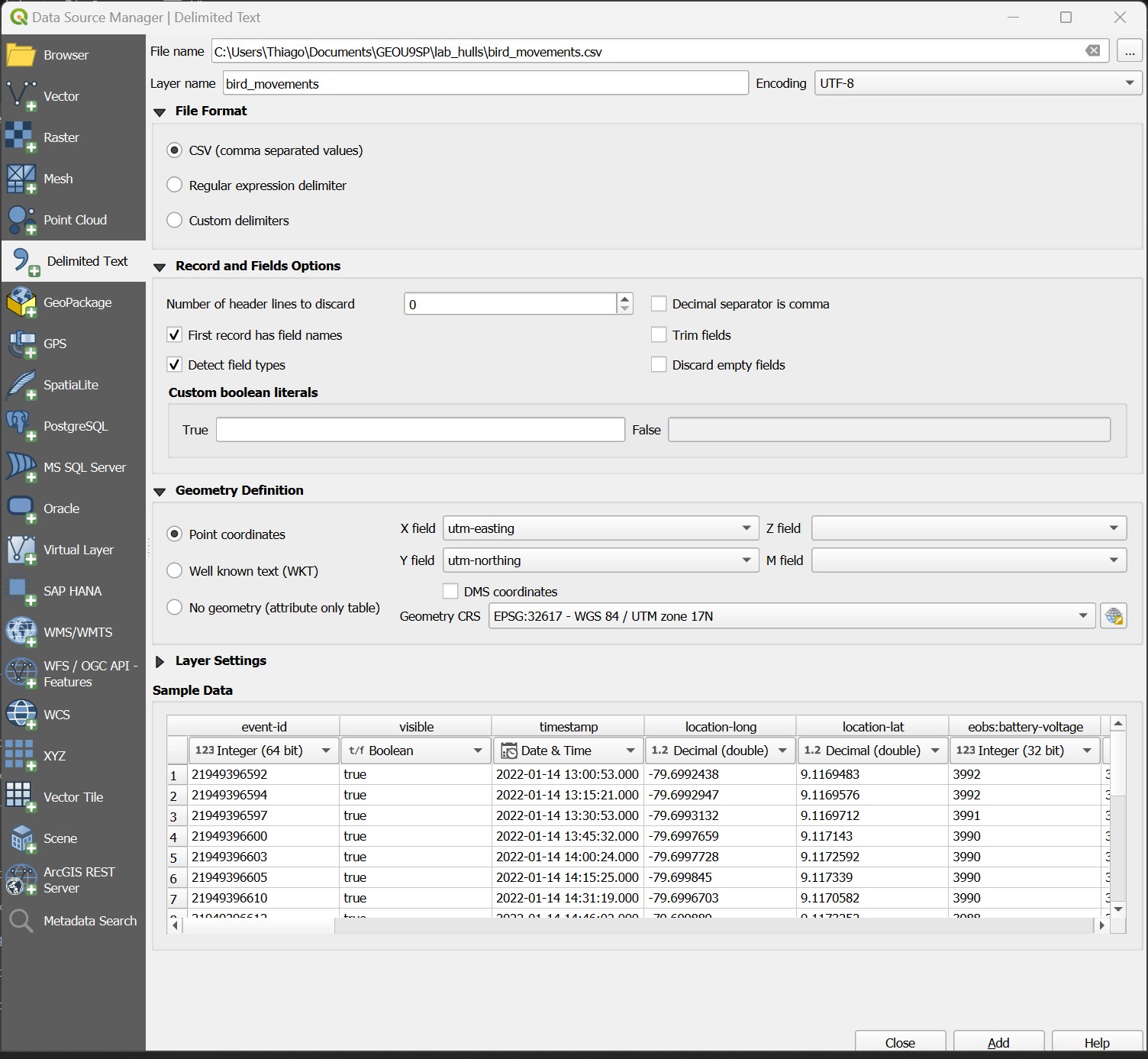
The file has both Latitude Longitude and Universal Transverse Mercator (UTM) coordinates, which are similar to British Grid coordinates, but for the entire world. UTM coordinates are ideal for field data that does not span large areas (you can read more about it here). We will use UTM coordinates since they are metric, and thus some automatic area calculations that will happen later will have the right units.

Now split the file into separate layers for each individual bird, saving each file as a separate geopackage (to preserve long field names) named as the individual_local_identifier tag (ex: Chachalaca_1.gpkg). Use Select by expression on the individual_local_identifierfield and then Export > Save selected features as... to create each subset.

Stop and Think

How many records, covering what timespan, are available for each individual bird?

Click for answer

To check it, you can use the Statistical Summary tool and the timestamp field you have created. Here are my calculations:

Chachalaca_1: 9731, 2022-01-14 to 2023-02-17
Chachalaca_2: 660, 2022-01-14 to 2022-03-19
Chachalaca_3: 2841, 2022-01-14 to 2023-02-17
Chachalaca_4: 3641, 2022-01-14 to 2023-02-18
Chesnut_1: 385, 2022-03-05 to 2023-02-17
Chensut_2: 296, 2022-03-18 to 2022-03-19
Keel-billed_1: 311, 2022-01-15 to 2022-02-09
Keel-billed_2: 1568, 2022-02-22 to 2023-02-18
Parrot_1: 41933, 2020-03-17 to 2022-04-18

14.2 Guided Exercise 2 - Convex Hulls

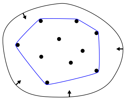
Convex hulls are a type of Minimum Enclosing Polygon. The best way to think of it is as if the points were pegs on a board, and you wrapped a stretch band around them. The convex hull is the shape with the smallest perimeter enclosing all points.

https://en.wikipedia.org/wiki/Convex_hull

In animal and movement research, convex hulls are commonly used to define species ranges or, for individuals, home ranges.

Important

There are two separate tools to calculate convex hulls in QGIS. The first is called Convex Hulls in Vector > Geoprocessing, but is usually NOT what you want. This tool calculates convex hulls for irregular polygons. To calculate convex hulls for points, you instead want to go to the Processing tab and then choose the Minimum Bounding Geometry tool under the Vector Geometry category.

For this exercise, we will first focus on the Chachalaca birds. We will also not consider Chachalaca_2 since it was only monitored for two months.

The first question we may want to ask as animal movement researchers is if there are well-defined territories for the birds, and if these territories overlap (i.e. do the birds interact?).

14.2.1 Calculating Convex Hulls

Go to the Processing tab and then launch the Minimum Bounding Geometry tool under the Vector Geometry category.

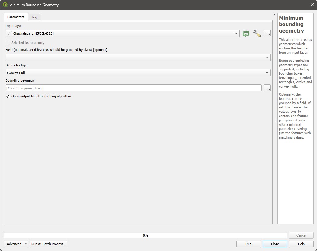
Select the Chachalaca_1 layer as Input Layer, and then Convex Hull for the Geometry Type (click on the Help button to see what each type of geometry represents). Save the file as Chachalaca_1_home_range.shp.
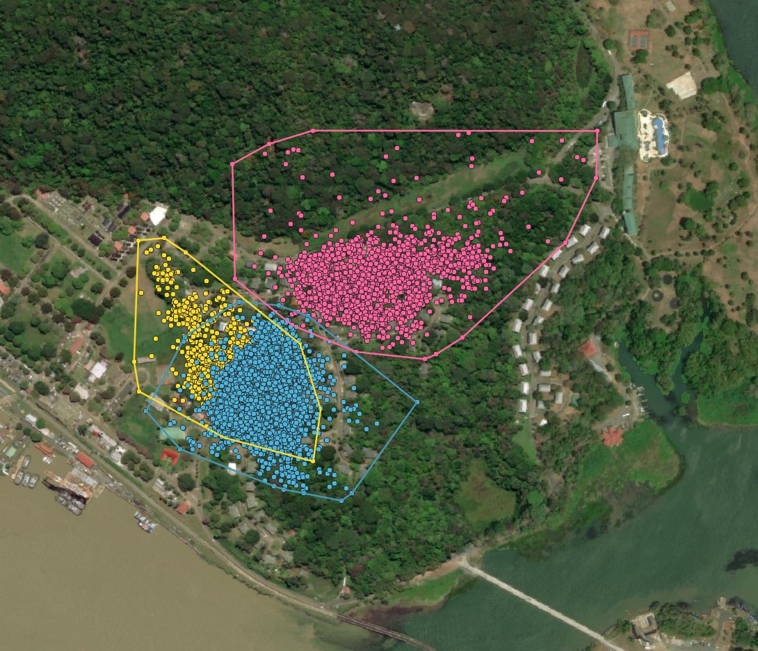
Repeat for Chachalaca_3 and Chachalaca_4.
Now set the home range polygon symbologies to an outline that is the same colour as the original points with no fill (or a transparent fill), to evaluate the overlap in home ranges. Also add the ESRI Satellite Layer from the QuickMap Plugin for reference. Mine looks like this:

Stop and Think

Now using the Geoprocessing tools you have learned, calculate the amount of percent overlap between each home range. Based on this, which individuals may be interacting with each other?

Click for answer

First you need to recalculate the areas in proper units. The Convex Hull tool calculates the area using the layer units, which for this dataset are degrees.

You can use the Intersection tool to find the overlap between home ranges. You need to calculate it two times for Chachalaca_1 x Chachalaca_3 and Chachalaca_1 x Chachalaca_4. You can see from the previous step that Chachalaca_3 and Chachalaca_4 do not overlap, so no need to calculate it.

The intersection polygons will have the area fields from both original layers (one of them renamed as area_2), and you can use the Field Calculator to calculate the area of the intersection.

C1: 121393 m $^{2}$
C3: 91856 m $^{2}$
C4: 230018 m $^{2}$
C1 x C3: 59654 m $^{2}$ (49% of C1 and 65% of C3)
C1 x C4: 2867 m $^{2}$ (2.3% of C1 and 1.2% of C4)

So we can conclude that Chachalaca 1 and 3 interacted very often, Chachalaca 1 and 4 interacted more rarely, and Chachalaca 3 and 4 did not interact at all during the study.

14.3 Guided Exercise 3 - Habitat Use

The second question we may want to explore is what the main types of habitats each bird is using are. For that, we can use the convex hulls that determine our home ranges, and the land cover layer included in the dataset. The data documentation includes a table with a key for each land cover type.

Stop and Think

Using the tools you already know, determine which habitats comprise each Chachalaca home range, and their respective area.

Click for answer

We have the home ranges as polygons, and the land cover dataset as a raster. There are thus two ways of achieving this. One is to Polygonize the raster, and then use Clip to cut the resulting vector land cover map by each of the home ranges, and then recalculate the areas of each habitat using the Field Calculator. The second is to cut the raster by each of the home ranges using Extract by Mask Layer, and then use Raster Layer Unique Values Report in the Processing panel. These are the values I got using the second option (fewer steps):

Chachalaca 1: Class 7 (Built Area) = 106800m $^{2}$ ; Class 2 (Trees) = 14400m $^{2}$

Chachalaca 3: Class 7 (Built Area) = 85900m $^{2}$ ; Class 11 (Rangeland) = 6200m $^{2}$

Chachalaca 4: Class 2 (Trees) = 151600m $^{2}$ ; Class 7 (Built Area) = 79900m $^{2}$

So we can see that while Chachalaca 1 and 3 have decided to explore mainly urban habitats, Chachalaca 4 is mainly exploring the forest habitat, indicating possible behavioural adaptations and/or territoriality.

14.3.1 Guided Exercise 4 - Creating temporal animations with QGIS

QGIS includes a feature called Temporal Layers, which allow us to animate the layers following time stamp information, to see how patterns change over time. We will use it now to look at the Chachalaca movement in time.

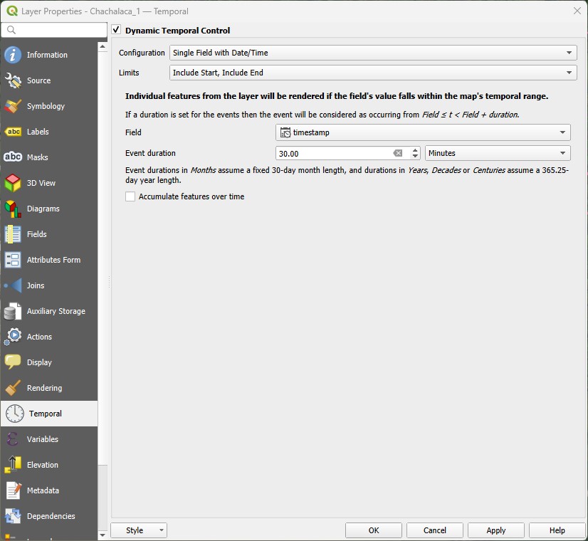
First, select the Chachalaca_1 point layer and go to Properties > Temporal. Then check the Dynamic Temporal Control box, and select Single Field with Date/Time as the Configurations, and Include Start, Include End as Limit. Then pick the timestamp field for Field, and set the event duration to 30 minutes (the minimum duration as per our metadata). Click in Apply, then OK. A clock symbol will appear to the right of the layer name to indicate it is time-enabled.

Now repeat the process for Chachalaca_3 and Chachalaca_4.
Now launch the Temporal Controller Panel () from the main QGIS toolbar. It will look like the panel below. If it looks different, make sure you click on the Animated Temporal Navigation button (small green play button within a circle).

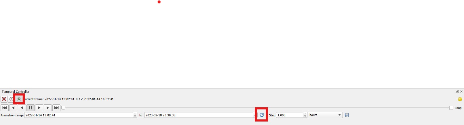
Then calculate the time range for all time-enabled layers by clicking on the button with two blue arrows. Set the Step to 1 hour, and then press the back play button. You will see Chachalaca_1 and Chachalaca_3 at first (remember there is no recording during the night, so there will be some periods with no points).
Now pause the animation, click on the double back-arrow to return to the start, and then change the Step to 1 day. Notice how even though Chachalaca 1 and 3 have a lot of overlap in their home ranges - on a daily basis they tend to mostly stay away from each other, seldom crossing paths. Also notice how Chachalaca 4 really tends to keep within the trees, rarely venturing into open areas.
Now pause and reset again, and then set the Step to One week. Notice how Chachalaca 4 tends to avoid crossing the big open patch that divides its home range, and only sometimes ventures into the northern area.
Pause and reset the animation again. Then launch the Windows Snipping Tool by going to the Start Menu and then typing its name (see here for Mac).

It will look like this:

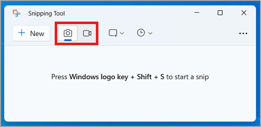
Read this entire section before doing it. Change the snip type from image (photo camera) to video (video camera), Then click on New. Drag the mouse to capture the map area of QGIS, and then click on Start Recording. There will be a countdown from 3, and then the recording will start. Once it starts, press the play button in QGIS to start the animation, and let it run through. Then stop the recording.

You should now have a video recording that could be used on a presentation! Here is mine (press the play button!)

Video Player is loading.

Current Time 0:00

Duration -:-

Loaded: 0%

Stream Type LIVE

Remaining Time -:-

You could also use the Export Animation function of QGIS by clicking on the Disk icon of the Temporal Controller. What it does however is saving each animation frame as one separate image, which you need to combine into a video later using video creation software, or as an animated GIF using an online tool such as EZGIF:

Congratulations, we have reached the end of the GIS content we are covering this module (with the exception of using GPS receivers). Well done! You should now feel confident in using the tools you have learned to solve spatial problems, and also comfortable learning new tools independently as the need arises. Good luck on you GIS journey!

And stay spatial!