1 Lab 1: QGIS overview and file management
The purpose of this lab is to give you a first overview of what a proper GIS workflow looks like, from start to end. As you progress on your exercises the projects will become more complex, but the general workflow will not change.
Developing proper project and file management habits from the start is the best thing you can do to succeed in GIS. Speaking as someone who has been teaching and working with Geomatics for more than a decade, poor file/project management is the underlying cause of at least 50% of the GIS problems you may encounter.
1.1 Before you start!
Go through the Week 1 preparatory session on Canvas, and watch the seminar recording if you have missed it.
Read this document to understand how the British National Grid indexing system works.
1.2 Guided Exercise 1 - Managing and loading files
In this exercise, you will download some data, prepare a folder structure to organise the files in your GIS projects, then create a QGIS project file and add some GIS data to it.
1.2.1 Downloading the required data
For this practical you will use the “OS open road” and “OS Terrain 50 Digital Terrain Model” spatial datasets, specifically for the NS89 tile of the Ordnance Survey British National Grid. (Read about what these datasets are here: OS Open Roads , OS Terrain 50).
Head to the Digimap website, and if you haven’t already, make sure you accept the user licenses for all datasets, as show on the instructions video available on Canvas.
Go the
Ordnance Surveysection of the site, and then pick theView maps and download dataoption on the right.Following the steps shown on the instructions video, download the following datasets for the NS89 BNG tile only:
- OS Open Roads (under Vector Data) - choose the
SHPformat - “OS Terrain 50 Digital Terrain Model” (NOT Terrain 5 and NOT Contours!, under Land and Height Data) - choose the
ASCformat
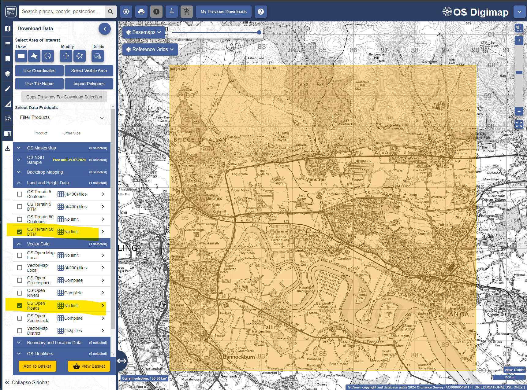
If you have correctly searched for tile NS89 and checked the required datasets, you will see a screen like the one below (the basemap may look a bit different). To enable the NS89 label on the tile, click on Reference Grid under Basemap (top left of the map canvas) and enable the 10km grid.
1.2.2 Creating a project structure
GIS projects generate a lot of different files, and quickly, so project organization is essential. The folder structure below is my personal suggestion for organizing GIS projects files and associated data. As you get comfortable managing your own projects, feel free to change the organization structure to something that best suits your own workflow and the specific project you are working on!
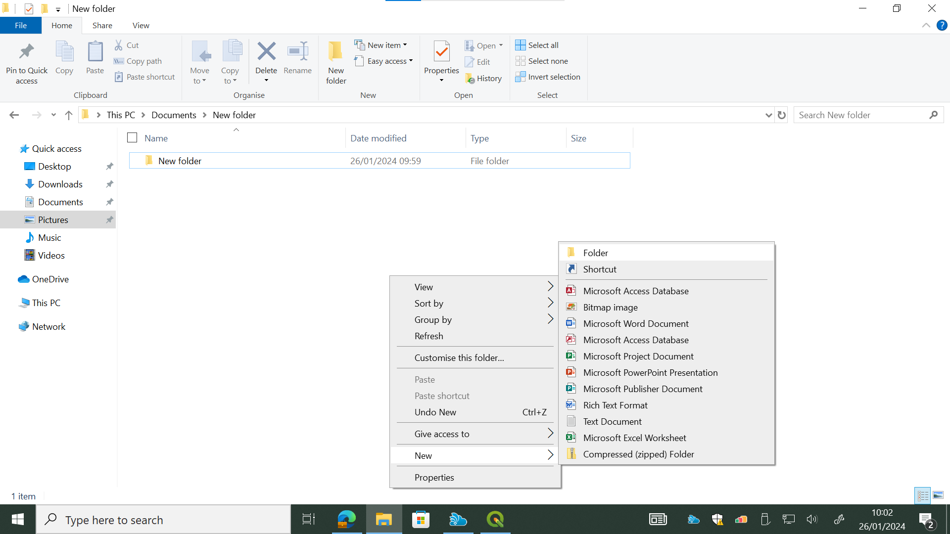
- Create a folder on your computer with the module name (
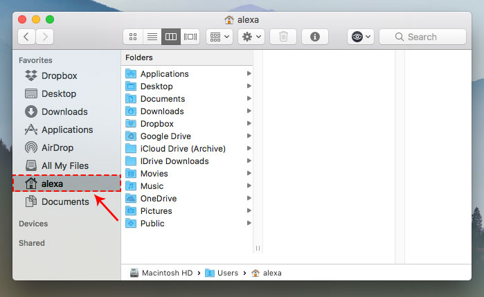
GEOU9SP), off of your main work folder. For Windows this will usually beDocuments. For Linux and Mac, create it on youhomefolder. (If you prefer and are comfortable with saving at another location on your computer, go for it!)
Windows:
mac OS:
Having complex file paths can sometimes create problems. That is why we try to keep our main projects on a base folder. If you would like to keep a copy of your data on your OneDrive folder you are encouraged to do so, but I don’t recommend working directly from it. That is because the full path to a OneDrive folder will to be very long and likely contain spaces. Mine, for example is
C:\Users\Thiago\OneDrive - University of Stirling\Documents. Those spaces in the name may create problems later. So I recommend instead to copy the completed lab data to your OneDrive folder at the end of each lab.For the same reason, never use spaces or special symbols on your folder and file names. Limit yourself to using letters A-Z and a-z, numbers 1-9 and just the underline (_) and dash (-) symbols.
Windows does not differentiate letter case, so if you create a file named
filename1.txtand then a second file namedFilename1.txtin the same folder, the second will overwrite the first. Mac OS does differentiate upper and lower case letters, soFilename1.txtandfilename1.txtare considered different names and can co-exist in the same folder.
Inside the new
GEOU9SPfolder, create a subfolder calledlab_1(notice I am avoiding spaces by using the underline)Inside
lab_1, create the following folder structure. On the diagram below, the folderrasteris a folder inside the folder01_raw_data, which is insidelab_1and so on.
.
└── GEOU9SP/
    └── lab_1/
        ├── 00_qgis
        ├── 01_raw_data/
        │   ├── raster
        │   └── vector
        ├── 02_processing
        ├── 03_final_products
        └── 04_notes
I like to start folder names start with double digits so they are kept in order. These folders will be used as follows:
00_qgis: we will use this folder to save our QGIS project files.01_raw_data: this folder will keep all the original data files you download. This way you can always go back to the start if something goes wrong. You can optionally use the sub-foldersvectorandrasterto easily know which kind of data you are working with, but this may not be necessary for small projects. As you obtain data you will create additional sub-folders for each individual dataset to keep data organized.02_processing: here we will keep all the intermediate files you generate as part of your work. Make ample use of sub-folders to identify each step of the workflow.03_final_products: here we will keep the final products of our intended analysis. This makes it easy for us to find the latest version of our final results, without risking confusing it with intermediate files. This can also include maps, reports and any other ‘deliverable’ resulting from your analysis.04_notes: here we will keep all our non-GIS files. For example, it may be a good idea to keep a text file documenting the project steps as you work on it. You could also save here screen grabs of specific steps. Again, use sub-folders as needed to keep your data tidy.
- Now move the data you’ve downloaded into your organized project folders and extract (unzip) them if necessary. The terrain data folder (
terrain-50-dtm_xxxxxxx) should go into therasterfolder within01_raw_dataand the roads folder (open-roads_xxxxxxx) into thevectorfolder. Thecitations_orders.xxxx.txtandcontents_order_xxxtext files should go into your04_notesfolder.
Each of the download datasets will contain several files once you unzip them. All of them are important, so make sure to keep them all together (except for the text files, these can go somewhere else).
Your folder structure should look like this:
.
└── GEOU9SP/
    └── lab_1/
        ├── 00_qgis
        ├── 01_raw_data/
        │   ├── raster/
        │   │   └── OS_terrain_50/
        │   │       └── ...
        │   └── vector/
        │       └── OS_roads/
        │           └── ...
        ├── 02_processing
        ├── 03_final_products
└── 04_notesWhat are the citations_orders.xxxx.txt and contents_order_xxx files? What information do they contain?
- Start a new text file (a Word .doc file or a Notepad .txt file) in your
04_notesfolder, and write a few lines documenting the steps you took until now. If you prefer handwritten notes on a paper notebook, feel free to use it instead! The important thing is to keep track of the steps you are taking. As projects get more complicated, it is easy to forget which steps we took, and in what order!
1.2.3 Creating a QGIS project and adding data to it
A QGIS project is a file, which will remember all the data layers you have loaded, their stacking order, the styling of each layer, and some other information such as the coordinate reference system. It will also keep any map layouts that you create. But he project file will NOT store the data files themselves!!. It will only link to the data. That is why we need good project folder organisation. If a data file is moved or renamed, the QGIS project file will lose track of it.
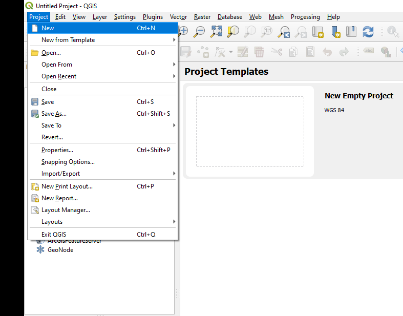
- Open QGIS. Then create a new project in QGIS by clicking on
Project > New...or pressing Ctrl-N:
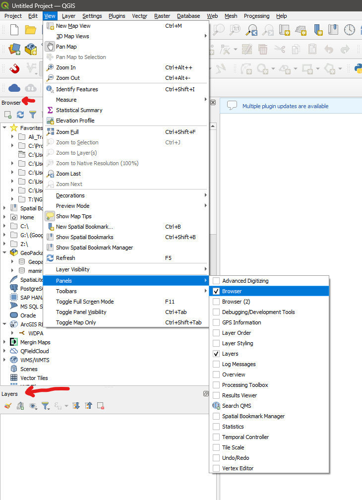
If you start QGIS and you don’t see the Browser and Layers panels to the left (like the figure below), then go to the menu View > Panels and then enable the Browser panel. Then repeat, this time enabling the Layers panel.
Add to your project the layers
NS_RoadLink.shpfrom the OS Roads dataset and theNS89.ascterrain data from your organized project folders. Don’t worry if the extents don’t match - it’s just that the OS DEM and the OS Roads are distributed in different sized ‘chunks’.Save your project inside the
00_qgisfolder. You can save your project by clicking on the Save button, going toProject > Savemenu, or by holding the keysCtrl+S (Command+S on Mac).Open the project settings by clicking on the menu
Project > Properties.... You will then see this window:
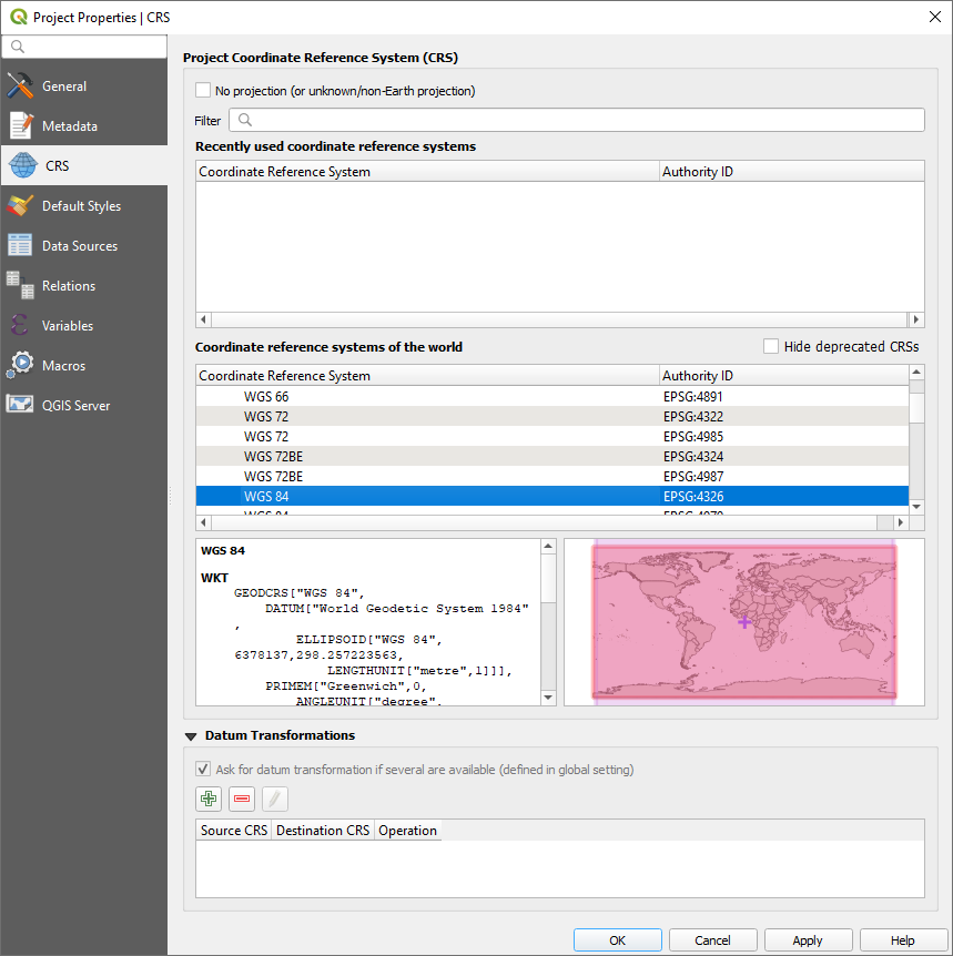
The main things to set on your new project are the project home folder, the coordinate reference system (CRS) and the measurement units.
As the project home on the
Generaltab, select thelab_1folder you created. This helps quick navigation when opening and saving data.For measurement units, make sure distance units are set in meters, and area units in squared meters, also on the
Generaltab. Any QGIS operations that calculate distances or areas will use the units set by the project.
- For the CRS, go to the
CRStab (to the left) and search for 27700 in theFilterbox. That is the EPSG code that identifies the OSGB 1936 British National Grid coordinate reference system (CRS). Select it by clicking on it - you may need to expand your search results by clicking on the small arrows besidesProjectedandTransverse Mercator.
EPSG stands for “European Petroleum Survey Group”, and designates a database with standard codes for hundreds of coordinate reference systems. Over time, you will probably memorize the EPSG codes for the CRSs you use more often.
- Save your project again.
1.3 Guided Exercise 2 - Organizing and styling your layers
One of the most powerful aspects of GIS software is the ability to style spatial data in very specific ways, by specifying colours, line widths, line types, symbols, etc. As we progress in the module you will learn more and more ways to style your data.
On the
Layers panelto the left of the screen, select theNS89layer, and drag it to the bottom of the layers list if not there already.Turn the roads layer off for now, by unchecking the box besides its name.
Right-click on the
NS89layer name and chooseRename Layer. Rename it toDigital Elevation Model (50m).Open the file explorer in your system, and find the
NS89.ascfile that holds the actual elevation data, which you downloaded from Digimap.
Will changing a layer name in the layer panel also change the name of the source data file for that layer?
Right click on the newly renamed terrain layer and choose
Zoom to Layer. This is a very handy tool to “find yourself” if you end up zooming or panning the map too far.Right click on the terrain layer name again and select
Properties..., then go to theSymbologytab.On the
MinandMaxboxes, type0and500respectively. This determines the range of layer values to be visualised.Select
Rendering typeto beSingle Band Pseudocolor, and change theColor rampoption by clicking on the down-arrow button to the right and picking thespectralcolour ramp. If you click on the colour ramp itself it will open a new window to customise it. This is now what we need for now, so just close it and use the down-arrow.Click on
Classify(under the drop down menu that says * Mode: continuous*). The colours will be matched to the range of elevation values in the layer.Click again on the little down-arrow button beside the colour palette button and select
Invert Color Rampat the top of the options, so that the lowest heights are coloured blue. Then click onOK.Note how the legend for you terrain layer has changed on the Layers panel. It now shows the minimum and maximum elevations and the colour ramp. Save your project.
Why do we bother inverting the colour ramp for this dataset?
Rename the
NS_RoadLinklayer toRoad Network.Go to its
Symbologyproperties, like you did for the terrain layer, Notice that the symbology options are data-specific (vector vs. raster). SelectSimple Linein the symbology window (under the mainLineoption). Then under the window, go to theColoroption an click on the down-arrow menu to change the line colour to a dark grey. If you click on the actual colour, a more complex colour-picking window will appear. You can use either the quicker colour drop down or the main colour window, whatever you prefer.Change the
Stroke width(line width) to 0.3. ClickOK. Reactivate the layer if needed to visualise it.
1.4 Guided Exercise 3: Processing data using GIS operations
The core of GIS work is to use the many built-in operations (also known as functions or tools) of GIS software to process the data in some way, and thus create additional information. For this exercise, we will use an operation that creates a new layer representing the boundaries of the terrain data layer, and then use a second operation to cut the roads layer to the same shape and extent as this new layer.
Go to the
Vectormenu and selectResearch Tools > Extract Layer Extent.... Select the terrain layer as yourInput layer, and clickRunto generate a temporary layer. Temporary layers are not kept once you close QGIS, unless you save it manually later. TheExtract Layer Extentwindow will not close automatically after you run the operation, so click onClosewhen you are done.Go to
Vector > Geoprocessing Tools > Clip.... Select the roads layer as theInput Layerand the new temporary layer as theOverlay Layer.This time, we will save the output. Click on the
...button to the right of theClippedtext box, and then chooseSave to file. Save your new layer on the folderGEOU9SP/lab_1/02_processing/, naming itclipped_roads.shp. Make sure theSHP fileformat is selected below the file name. Then click onRunto execute the operation. Close the window.Turn the original roads layer on and off to see the result of your operation. Then right-click on the original roads layer, and select
Styles > Copy Style > All Style Categories. Then right click on the new (Clipped) roads layer and selectStyles > Paste Style > All Style Categories. This is a great way to style several layers in the same way without effort.Remove the original roads layer from your project by right clicking on it and selecting
Remove Layer..., and then rename you clipped layer to “Roads”. Save your project.Close QGIS. It will give you a warning - read it carefully and then confirm it.
Reopen QGIS, and load your project again. Notice it remembers exactly where you last saved it, including zoom level, layer names and layer styles. The “Extent” layer will still be on your list but will appear empty - it has been deleted once you closed QGIS. Remove it from the project and save again.
What are the names of the two GIS functions you just used in this exercise?
Why did you have to create a new layer representing the extent of the terrain data before clipping the roads layer?
What does the warning given by QGIS when you closed your project mean?
1.5 Guided Exercise 4: Creating a map layout
The main QGIS interface (or any other GIS software) is developed and optimised for interactive work. But very often as part of our GIS analysis we will want to generate nice maps and figures following proper design rules (and not just grabbing a screen capture of the QGIS window and dumping it on a page - hint for your assignment reports). For that, we use the QGIS Map Layout Editor.
Click on
Project > New Print Layoutand name itLab 1 Layout. A new window will open showing the QGIS Layout Editor. Notice that the main QGIS window remains open as well. These windows are ‘linked’, so that the map layout reflects any styling changes you make on the main window.The
Layoutwindow often opens at a small size. Maximize it so it takes the whole screen, and use your mouse wheel to zoom into the blank page until it occupies most of the canvas.Add a new map to the layout by clicking on the
 icon. Drag it through the page so it covers about 2/3 of it horizontally, and the full height of the page (minus some borders).
Use the
Interactive Extenttool to pan (click and drag) and zoom (mouse wheel) until your data covers the entire map box. But make sure you don’t hide the edges of the data by zooming in too much!
Now fine tune the map scale by changing the
Scalevalue on the bottom right panel. Remember that this value means “1:value”, i.e. one unit on the page is equal to that many units (value) in the real world. This means larger numbers will “zoom out”, and smaller numbers will “zoom in”. Try to make the map fill as much as possible of the map box, without clipping the edges.Go to the menu
Add Item > Add Legend...in the Map Layout Window (or guess the icon for this option on the side toolbar). Click the area beside the map box and drag to add a legend.Go back to the main QGIS window, right click on the terrain layer name, then select
Properties..., and on theSymbologytab, change theModeunder the class colour box toEqual Interval. Then select the number ofClassesto 10 (to the right of theEqual Intervalbox). Go back to the Map Layout editor.Go to the menu
Add Item > Add Scalebarin the Map Layout Window (or guess the icon for this option on the side toolbar). Click and drag in the area below the legend to add it to the map layout.Add a title to your map using the
Add Label...tool (either on theAdd Itemmenu or selecting the tool directly from the left sidebar). You can change the text by replacing the “Lorem ipsum” placeholder text with your own text on the left pane. Try to make it bold with a font size of 16 (hint: always use the down-arrow buttons for ‘quick settings’).Rearrange the items on the page until you are pleased with the results. Then go to
Layout > Export as PDF..., and export your map, naming it properly and saving it onGEOU9SP/lab_1/final_products. It is a good idea to export as PDF if you want your map to be a standalone document. If you are exporting to insert the map into a report, then useLayout > Export as Image...instead.
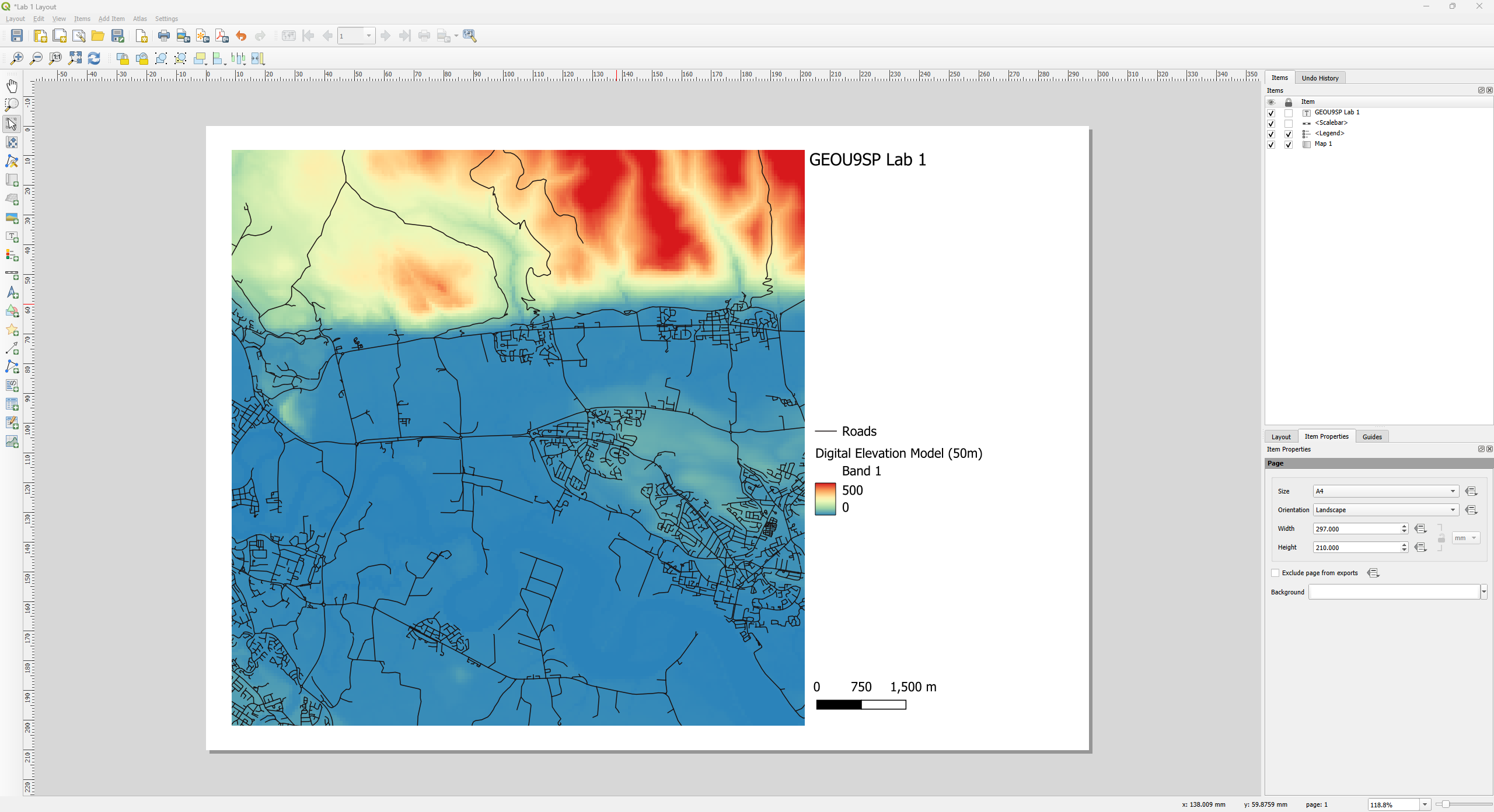
For reference, my map looked like this at this stage:
- Then close the Map Layout window, save your project on the main QGIS window, and close QGIS. Reopen QGIS, and go to
Project > Layout Manager. The layout you created previously should appear on the list. Select it and click onShowto reopen the Map Layout window.
Congratulations! You have successfully finished your first GIS project, using proper file management practices! As a final suggestion, create a “workflow_notes” file on GEOU9SP/lab1/notes and write up a quick overview of what you did, along with any specific notes you would like to remember later.
1.6 Independent Exercise 1
At the end of each lab, you will have the opportunity to reinforce what you learned by going through ‘independent’ exercises. These will use the same operations you learned with the guided exercises, but it may require you to figure out small bits of new functionality and will not have step by step instructions.
As the module progresses, the independent exercises will give you less and less directions, to reflect real-world GIS usage. Don’t skipe the independent exercises - it is easy to fall into a false sense of ‘I got this’ when only following step-by-step directions.
Create a new project folder structure for this project, under your main GEOU9SP work folder.
Download the zipfile containing the Air Photo Mosaic and the Stirling Council Geospatial Data from here.
Extract the data from the zipfiles and move them to the proper project folders.
Open QGIS and create a new project that uses the OSGB British Grid (EPSG 27700) coordinate reference system.
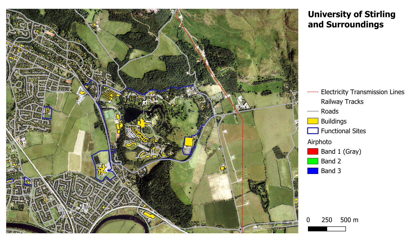
Import the airphoto raster image and the vector files for Buildings, Roads, Railway Track, Electricity Transmission Lines, and Functional Sites into your QGIS project.
Organize your layers so that, from top to bottom, you have transmission lines, railways, roads, buildings, functional sites, and then the airphoto image.
Style your layers so that transmission lines are styled as thin dashed red lines, railways as thick white lines, roads as thick grey lines, buildings as filled yellow polygons and functional sites with a thick dark blue outline and no fill colour (hint: check the
Fill styleoptions).Clipall your vector layers to the extent of the airphoto image.Create a map layout covering the entire extent of the airphoto. Add a title, legend and scale bar to your layout and export it as a PNG image. Then insert your exported file as a figure into a MS Word document.
- Now answer the questions below:
How far is the Pathfoot Building from the Cottrell Building? Calculate it both “as the crow flies” (linear distance) and as if you were walking. (Hint: use the Measuring tool
 ).
).What is the total surface area of the water bodies in the University of Stirling Campus? (Hint: also the Measuring tool).
What is the classification of the UoS campus polygon within the “Functional Site” layer? (Hint: use the Identify Features tool
 ).
).