4  Lab 4: Working with vector geometries

The purpose of this lab is to continue developing your knowledge about vector spatial data and vector-based GIS operations. Today you will learn how to make selections based on the overlap of two vector layers - called spatial selection, location selection or spatial query. This is a powerful way to combine data from different sources to generate new information.

4.1 Before you start!

1. Go through the Week 2 preparatory session on Canvas, and watch the seminar recording if you have missed it. Also make sure you have completed Lab 3.

4.2 Guided Exercise 1 - Spatial Queries

We will continue with the Earthquakes, Rivers and Countries dataset from the previous lab.

1. If you have zipped your project from the last session, just unzip it and get to work. If not, then download the data again, and redo your project organization. As a reminder, the files to be loaded are: global_earthquakes_2011.gpkg, MajorRivers.shp, and ne_50m_admin_0_countries.shp.

For our next step in the analysis, we would like to focus only on earthquakes on land (i.e. not ocean). This information is not contained in the Earthquakes layer, but we do have a Countries layer that separates land from ocean. Could we use that to make a selection?

2. Go to the menu Vector > Research Tools > Select by Location..., or click on the button on the main QGIS toolbar. You will get this window:

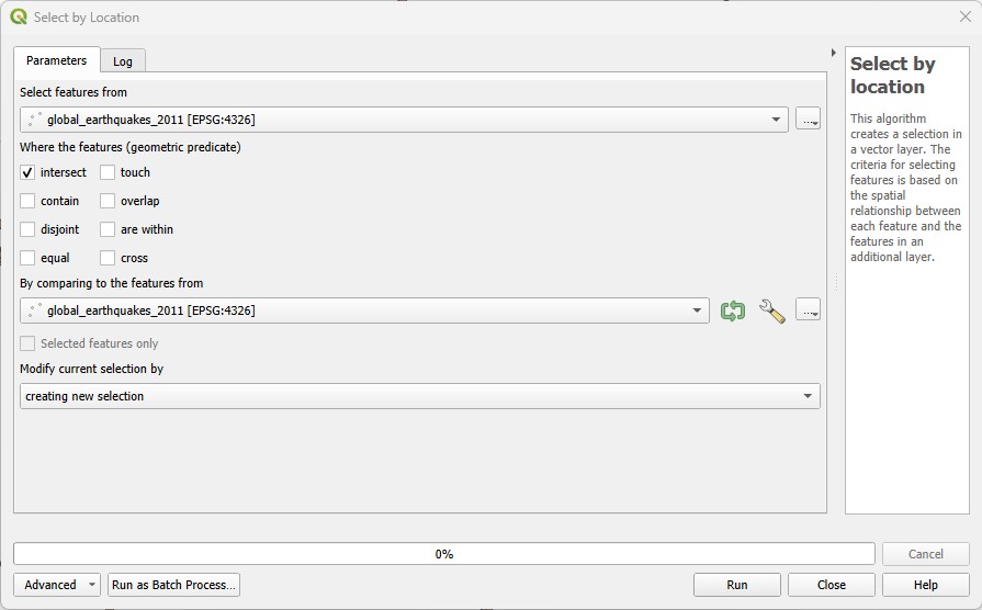
3. Select the Earthquakes layer as Select features from. Then check only the Are within query option. Then pick your World Countries layer for By comparing to the features from. Click Run, and after it is finished, click Close.

4. Visually inspect the results of your selection, and then open the Attribute Table for the Earthquakes layer.

Stop and Think

How many Earthquakes were originated on land in 2011?

Click for answer

3742 earthquakes.

Now that we identified the earthquakes on the continents, we may want to add this information to the Earthquakes layer as an attribute, in case we need the information later.

5. Still on the Attribute Table of the Earthquakes layer, open the Field Calculator, and create a new Text(string) field called Origin. Make sure the option Only update selected features is enabled this time. Then on the Expression window, just write 'Land'. That means the word Land will be added as the attribute value for every selected feature.

6. Now back on the Attribute Table window, click on the Invert Selection button ().

7. Return to the Field Calculator and this time use the Update Existing Field option to the right, instead of Create a new field. Make sure the option Only update selected features is still enabled. Pick Origin as the field to be updated, and now just write 'Ocean' on the Expression window. Click OK.

8. Now use the Origin attribute to style the colour or shape of your Earthquake points differently for land and ocean, using the Symbology options. Pick the Categorized symbology option at the top, set the Value to the Origin attribute, and then Classify.

Stop and Think

Do you understand why you did the steps above?

Click for answer

We wanted to create a new string attribute designating an Earthquake as either Ocean or Land. But the information on where the Earthquake is depends on whether it overlaps with the Countries layer. So we need to combine select by location with the Field Calculator. First we create a selection of land quakes based on location, and then we add a new field to the Earthquakes layer, to be filled with the word Land. But since we checked the Only update selected features option, only the selected features will be filled, and the rest will remain blank (Null). We then invert our selection so that only ocean quakes are selected, and update the existing field by filling in the word Ocean just for these selected features.

Creating this new attribute adds the possibility of styling the points by Origin, which would not be possible just based on the selection.

Now, let us find details about earthquake originating on a specific continent.

9. On the World layer, use Attribute selection (as in Exercise 3) to select all countries from South America. Then go to Vector > Research Tools > Select by Location... and select all Earthquakes that are within the Countries layer (same process as above), but this time make sure you turn on the option Selected features only.

10. Another way to make a selection ‘permanent’ is to export it as a new layer. While you still have the above selection on, right-click on the Earthquakes layer name and choose Export > Save selected features as.... Name your exported file as Land_earthquakes_2011_south_america. Choose an appropriate folder to save it within your project structure by clicking on the ... button to the left of the file name box, and select your format of choice (geopackage or shapefile). Click on OK. Save your project.

4.3 Guided Exercise 2 - Geometry-based attribute calculations

Another way to relate geometries to attributes is when we want to store some property of the geometry as an attribute itself, such as area, length or perimeter. QGIS also has tools for that.

As an example, let us calculate the areas and border length (perimeter) of all the World’s countries.

11. Before using any of the geometry-based operators, we need to set up our desired units for the project. Go to the menu File > Properties... to open your project properties. Then on the General tab, set the Units for distance measurement to Kilometers and the Units for area measurement to Square Kilometers (yes, we will use SI units because we are scientists!).

It is always important to think about your problem before choosing the units for length and area calculations. In this case, using the default of meters and squared meters would not make sense for things as large as countries.

12. Now open the Attribute Table for the Countries layer and launch the Field Calculator. Create a new attribute called Area_km2 (it is always a good idea to add the units to the name to avoid any confusion) that is a decimal number with two decimal places. Then on the centre panel, find and expand the Geometry heading, and double click on the $area option to add it to the expression window. Then click on OK to calculate the field.

13. Remember to deactivate editing mode!

Stop and Think

1. What is the difference between $area and area? Hint: look at the help text on the right panel.

2. Why should we use $area instead of area here?

Click for answer

1. The $area operator calculates geodesic area, meaning it takes into consideration the curved surface of the ellipsoid (defined by the projects CRS). It will also use the units specified in the project properties. The area operator will calculate planimetric area (i.e. a flat surface) and will derive the units from the CRS of the layer.

2. Since we are calculating very large areas, geodesic area will be more correct than planimetric area (unless the dataset uses an equal-area map projection). Moreover, the data is in EPSG24326 (WGS 84), which has degrees as units. If we used area we would get areas in squared degrees, which don’t make a lot of sense.

14. Now repeat the process above, and calculate Per_km as a new attribute, using the $perimeter operator (we use it instead of perimeter for the same reason above).

Stop and Think

The perimeter/area (PA) ratio is often used as a measurement of polygon complexity. Can you answer which country has the most complex border in the world?

Click for answer

Use the Field Calculator to calculate areas and perimeters (you just did), then use it to create a new PA_ratio attribute (decimal number) using the expression "Per_km" / "Area_km2" (assuming these are the attribute names you used). Then use the Summary Statistics tool to find the maximum PA_ratio value in the dataset (4.592). The use Select by expression to select which feature has "PA_ratio" = 4.592. That would be the Vatican! A quicker way to answer this (that only works for min/max values) is to click on thePA_ratio` attribute name on the Attribute Table twice, to sort it in ascending and then descending order, and then checking which country is the top row after sorting.

Good job! You now know all you need to query, create, delete, update and summarise attributes. You will use these tools a lot whenever you are doing any GIS work, so it is important to know them well.

To further solidify your knowledge, do the Independent Exercise below, which reviews all your learning from the past week and this week.

4.4 Independent Exercise - Supporting Wildcat conservation in Scotland.

You want to investigate how priority areas for wildcat conservation (WPAs) overlap with protected areas, and the risk of wildcat roadkill.

For that, obtain the following layers from the NatureScot Open Data Hub. Get them in either shapefile or geopackage format.

• Wildcat Priority Areas (WPA)
• Sites of Special Scientific Interest (SSSI)

Then obtain the Open Roads layer for all of the UK from the Ordnance Survey OS Open Data hub, also as a geopackage (it is a large file and it may take a while to download).

Finally, obtain the UK country boundaries from the Global Administrative Boundaries (GADM) hub. Get the GeoJSON file at Level 1 (Level 0 is the UK border without countries, level 1 is countries, level 2 is counties/council areas, etc.)

Organize the data and create a new project where you load all four datasets. Order and style them as you prefer. Then:

1. Answer the questions:

   1. What is the data model of each layer?
   2. What is the file format of each layer?
   3. What is the CRS of each layer?
   4. How many features does the WPA dataset have?
   5. How many attributes does the WPA dataset have?

2. The UK boundaries file has a different CRS from the rest, and it also contains all countries. Reproject this layer to the same CRS as the other layers, and then create a new layer containing the Scotland boundary only. Remove the UK layer from the project after that.

3. The roads layer covers all of the UK, making it very heavy and slow to use. But our analysis concerns Scotland only, so create a new layer containing only the road links (lines) inside the Scottish boundaries. Remove the full UK layer from the project after that.

4. The attribute Shape_Area of the WPA dataset does not indicate any units. It is always useful to have field names that hint at the unit for the values, making the data more self-explanatory. Recalculate the area of each WPA in square km, naming the new field ‘Area_km2’. Then delete the ‘Shape_Area’ attribute from the dataset to avoid confusion for future users.

5. The Sites of Specific Scientific Interest (SSSIs) are a category of protected area in Scotland. These may offer additional protection to wildcats. Find all the SSSIs that overlap with WPAs, and create a new layer containing only these sites. Then calculate the total area of these SSSIs.

6. A major threat to wildlife is roadkill. Using the OS Open Data Open Roads dataset, answer the questions below:

   1. How many road segments overlap with WPAs? (Create a new layer containing only, the selected data, to use below).

   2. What is the total length of roads within WPAs?

   3. Not all roads present the same risk. In the UK, roads are classified as:

      • Motorways: high-speed expressways typically reserved for longer journeys between major cities;
      • A roads: major roads intended to provide large-scale transport links;
      • B roads: roads intended to connect different areas, and to feed traffic between A roads and smaller roads on the network;
      • Classified Unnumbered – smaller roads intended to connect together unclassified roads with A and B roads, and often linking a housing estate or a village to the rest of the network;
      • Unclassified – local roads intended for local traffic. The vast majority (60%) of roads in the UK fall within this category.

What is the total length per road class for all roads intersecting WPAs?

You will notice a ‘problem’ with the terms used in the road classification attribute - its unique values don’t match the terms above. You will need to create a new field called class_fix that keeps the classification of Motorway A, B, Classified Unnumbered and Unclassified unchanged, but changes the records labelled as both Not Classified and Unknown to Unclassified.

4. Along with road class, the length of the road segment is also important in determining overall traffic speed. To take that into consideration, select all roads within WPAs that are of either Motorway, A or B class and have 100m or more in length. Create a new layer from this selection.

5. GIS analyses will almost always have a visual component, as maps are a natural way to tell a ‘spatial story’. To finalise your exercise, organise and style your layers to show, in the most readable way possible (i.e. think about orders, line colours, widths and styles, fill colours, etc):

• The Scottish boundary;
• The WPAs;
• The boundaries of the SSSIs, distinguishing between those that do and do not overlap with WPAs;
• All Scottish roads differentiated by class using line width;
• All the road segments that are Motorways, A or B roads within WPAs which are longer than 100m. These should use the same line widths as above to differentiate road class but have a different colour from other roads.